Guides / Excel
Compare Two Columns in Excel: Matches & Missing Values
To compare two lists in Excel, use COUNTIF to check whether each value appears anywhere in the other column. Check both directions to find missing values, or highlight the matches. You can also paste or import your columns into our browser tool without writing formulas.
Using Google Sheets? Follow the Google Sheets column comparison guide for its formulas, filters and conditional formatting steps.
Choose your method
Compare the same row or search the whole list?
Use =A2=B2 when each row is already aligned and you want to compare those two cells. It returns TRUE or FALSE and does not distinguish uppercase from lowercase text. =EXACT(A2,B2) also checks letter case.
When the lists are in different orders, a row-by-row comparison can miss a match farther down the other column. Use the COUNTIF method below to cross-reference the two lists by checking whether each item exists in the other list. Returning a related value from another column is a separate lookup task.
Find missing values between two Excel columns
Try this small example in a worksheet. Put List A in A1 and List B in B1, then enter the values below. Leave B5 empty.
| Excel row | Column A | Column B |
|---|---|---|
| 2 | SKU-A | SKU-B |
| 3 | SKU-B | SKU-D |
| 4 | SKU-C | SKU-A |
| 5 | SKU-A | empty |
Find items in A that are missing from B
- Type A checked against B in C1.
- Enter this formula in C2, then fill it down through C5:
=IF(A2="","",IF(COUNTIF($B$2:$B$4,A2)=0,"Missing from B","Found in B"))COUNTIF searches B2:B4 for A2. A count of zero means that item is missing from B. The first IF leaves the result empty when the input cell is blank.
Select A1:C5, choose Data → Filter, and filter column C to Missing from B. Only SKU-C in row 4 should remain. Clear the filter before the next step.
Check the other direction
Type B checked against A in D1. Enter this formula in D2 and fill it down through D4:
=IF(B2="","",IF(COUNTIF($A$2:$A$5,B2)=0,"Missing from A","Found in A"))Column D marks SKU-D in row 3 as Missing from A. Checking both directions matters: the first formula alone will not find this item.
For your own data, replace the last row in each lookup range and fill the helper formula down to the last input row. The $ signs keep the lookup range fixed while A2 or B2 changes as you fill down. These examples use English function names and commas; Excel may use localized function names or semicolons for your region.
Find matches and highlight them
Using the same example, filter column C to Found in B to see the matching rows from A. You should see rows 2, 3 and 5: SKU-A, SKU-B and SKU-A again. The two distinct shared values are SKU-A and SKU-B; the helper column keeps the original repeated rows.
To highlight matches in column A, clear any filter and:
- Select A2:A5, with A2 as the active cell.
- Choose Home → Conditional Formatting → New Rule → Use a formula to determine which cells to format.
- Enter the formula below, choose a fill color in Format, then confirm. Check that Applies to is
=$A$2:$A$5.
=AND(A2<>"",COUNTIF($B$2:$B$4,A2)>0)A2, A3 and A5 should be highlighted. To highlight missing values instead, use the same rule with =0 in place of >0; only A4 should be highlighted.
The rule checks membership in the other column. Highlighting duplicate values across a combined selection can also flag repeats found only within one list, so it answers a different question.
Compare columns without formulas
Use our browser tool to check which names or IDs appear in one column, the other, or both. It compares list membership, not entire rows, quantities, or changes to Excel formulas. The tool example below uses different values to show how it preserves text identifiers and source references.
Compare your two columns → If you already have data in the tool, return to that original tab to keep working.
Watch the file workflow, one step at a time
These screenshots use the downloadable sample workbook linked at the end of this guide. It contains made-up text IDs. This is a separate file example from the short pasted lists below.
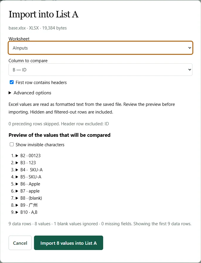
1. Import the workbook and select the ID column
Choose Import file for A, then select AInputs, B — ID and First row contains headers. Check the preview: A has 8 values and 1 blank row. Import them, then repeat for B with the same workbook, BInputs and the ID column. The Readme worksheet is not an input list.
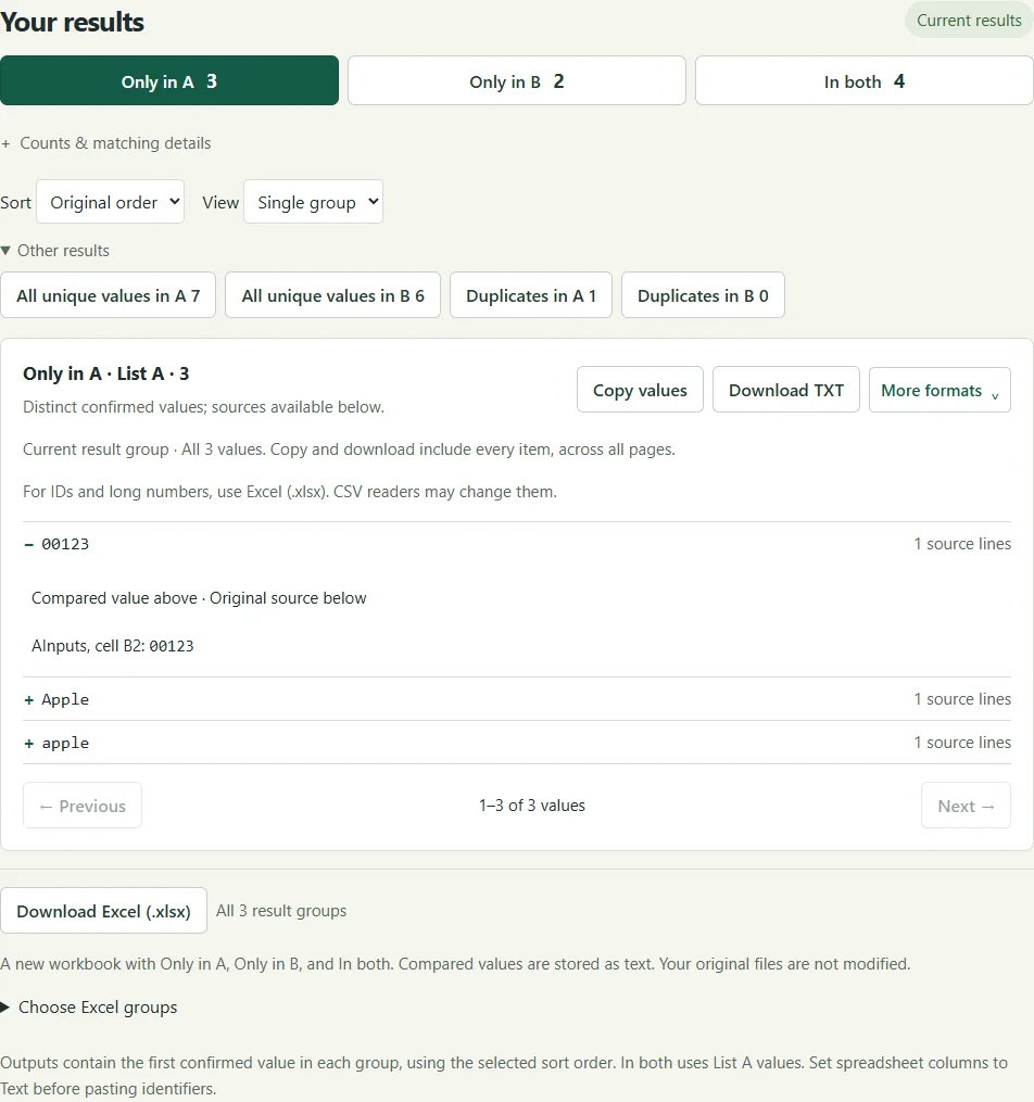
2. Compare and check a value against its source
Keep Trim outer whitespace on and Ignore case off. Choose Compare lists. This workbook produces 3 only in A, 2 only in B and 4 in both. Expand 00123 to find its original location, AInputs, cell B2. Apple and apple remain separate.
3. Download all three groups and check the workbook
Choose Download Excel (.xlsx). The new workbook contains Only in A, Only in B and In both. Excluding the Value header, check for 3, 2 and 4 rows respectively. Copy or TXT/CSV downloads can be used for a single complete group instead.

Compare your own columns → · Sample settings and expected results (new tab)
1. Choose how to add your columns
Paste one column into each list, or import a CSV or XLSX file and select one column for each side. Both routes use the same matching rules. List A and List B can come from different files or from two columns in the same file.
Paste one column at a time
Exclude headers and select cells without internal line breaks. Copy the first column into List A and the second into List B. Do not copy multiple columns. If tabs are detected, cancel and copy one column again, or explicitly keep every entire line as a single value. Commas remain part of a value unless you choose to split them with Clean up.
Import a CSV or Excel column
Choose TXT / CSV / Excel beside each list. For XLSX, select a worksheet, then choose one column. Review First row contains headers, the first 10 values, and the full row count. Advanced options let you set a starting row and CSV delimiter. Choose Import values to replace that list; cancelling keeps it unchanged. To compare two columns from the same workbook, select that file separately for A and B.
Excel values are read as formatted text from the saved file. Formatting can affect comparisons. Hidden and filtered-out rows are included. Saved formula results require confirmation and may be out of date; formulas are never calculated. A selected column with missing formula results, errors, merged data cells, or internal line breaks cannot be imported. Text identifiers retain their digits, but this tool cannot recover digits already lost in Excel.
Expand results to inspect CSV record and column numbers or XLSX worksheet and cell addresses. Imported columns stay read-only. Change selection reopens the preview; Edit as text removes original file references and uses input line numbers.
2. Check the rules and compare
Choose Try example → Load example in the tool, or paste these four lines into A:
00123
123
SKU-A
SKU-A
Paste these two lines into B:
123
SKU-B
Set Trim outer whitespace to on, Ignore case to off, and sorting to Original order. Choose Compare lists. These settings are explicit so you can reproduce the answer.
Matching options change which values belong together; they do not rewrite your original text. How matching rules and source references work →
3. Read the three main results
| Result | Values in this example |
|---|---|
| Only in A | 00123 and SKU-A |
| Only in B | SKU-B |
| In both | 123 |
A has 4 valid input lines and 3 distinct values. Expand SKU-A to check A's source lines 3 and 4. It appears once in the result: this does not tell you how many units are missing or why an item is absent.
If you copied from Excel row 201, the first pasted item is Input A, line 1 here. File imports instead show CSV record/column numbers or XLSX worksheet/cell references. Display wrapping does not create extra input lines.
4. Choose an output
Choose an output
Download Excel (.xlsx) creates a new workbook with three worksheets: Only in A, Only in B, and In both. Each contains a Value column with all compared values stored as text. Empty groups retain the header. It never changes the original workbook or includes other source columns.
Copy values, Download CSV, and Download TXT use the complete current result group, including values beyond the 100-item desktop or 50-item phone page. CSV includes a Value header, UTF-8 BOM and CRLF line endings. TXT and copying have no header and preserve the original result text. All input methods support every output format.
For IDs and long numbers, use Excel (.xlsx). CSV readers may change them. Formula-like CSV fields receive a protective apostrophe only after a disclosed confirmation; cancelling produces no file. That apostrophe remains data if you import the CSV again. TXT and clipboard output keep the original values; spreadsheet apps may interpret formulas or split tabs. Prefer XLSX for a text-preserving round trip.
Download starts in your browser; use Save file if a second click is needed. Check your browser's downloads or Files app: a triggered download does not prove it was saved or opened. Changes to inputs, rules, names or sorting invalidate old downloads.
Before pasting identifiers, format the destination spreadsheet column as Text. Your spreadsheet may otherwise convert leading zeros, long identifiers, dates or formula-like text. Check a few cells after opening the result. This guide does not claim a tested round trip in every spreadsheet version.
5. Check common problems
Why are 00123 and 123 different?
They are different text identifiers. Leading zeros are kept; digits already lost in a numeric source cell cannot be recovered.
Why does a repeated SKU appear only once?
Results count distinct values under your matching rules. One group can have several source records. Expand it to inspect them; use your original data for quantity reconciliation.
Why do two similar-looking values not match?
Check Trim outer whitespace and Ignore case, then inspect the original sources. Accents, punctuation and hidden characters can still differ; the tool does not normalize all Unicode. See the matching rules.
Can I change the imported column or edit its text?
Change selection reopens the file preview. Edit as text replaces file references with input line numbers. Changes make previous results out of date; compare again before copying or downloading.
Why was my file or selected column rejected?
Check UTF-8 encoding for CSV, ordinary unencrypted XLSX, the selected column, and the preview. Missing formula results, errors, merged data cells and internal line breaks are not supported. Oversized data is rejected rather than shortened. Review the file limits below and the message shown by the tool.
File limits
Each file and extracted list is limited to about 5.2 MB and each list to 100,000 data rows, including blanks and excluding a selected header. CSV must be UTF-8. Only ordinary unencrypted XLSX is supported, with at most 20 worksheets, 256 used columns per sheet and 500,000 populated cells per sheet. Expanded ZIP data is limited to about 52.4 MB total, about 21 MB per part and 2,000 parts. Oversized data is rejected rather than truncated.
Imports stop after 10 seconds; exports stop after 15 seconds or an output limit of about 33.6 MB. Excel text cells are limited to 32,767 UTF-16 units; unsupported control characters are rejected. TXT or CSV remains available where its format supports the text. No original file is overwritten, no other columns are exported, and no complete-row matching is performed.
Compare your two columns → · Read the complete matching and source rules
Try a sample you can check
The 9 October 2026 synthetic test by worktoolmap.com returned 3 / 2 / 4 distinct values in Only in A / Only in B / In both with trim on and case sensitivity on. The larger sample exported 125 / 125 / 125 values; every group was copied and its TXT, CSV and XLSX download reread.
For the base CSVs, enable the header option and select ID, the second column. For base.xlsx choose AInputs for A, BInputs for B and ID (column B). Expand 00123 to see CSV record 2, column 2 or AInputs, cell B2. Compare again after changing an input or a rule. These are text-cell samples, not evidence about numeric-cell recovery or formulas.
Download base workbook · Inputs, expected results and export checks (new tab)
Choose between an online list tool and an Excel workflow (new tab).